Constructionism and the new learning analytics

Bruce Sherin, bsherin@ northwestern.edu

School of education and Social Policy, Northwestern University

Introduction                                                                                      

Once upon a time, constructionism was fresh and new. In those early days, the world of education was a very different place. We needed to more than just sell educators on the constructionist vision; we needed to convince them that computers would one day be inexpensive enough, and ubiquitous enough, to be part of the everyday infrastructure of schools.

Today, it has been over three decades since Mindstorms was first published (Papert, 1980). The vision laid out there has proven to be remarkably resilient. Even now, the examples presented in Mindstorms evoke strong reactions, and they remind us of what education could be. But the world around us has been changing dramatically. It used to be a special day when a student had the opportunity to sit down in front of a computer. Now, it is increasingly the case that computers are seen as part of the basic infrastructure of learning.

This means that, although the constructionist vision might be largely unchanged, the larger world is different. The battles we have to fight are very different than those we fought only a short time go. It might also mean that there are new things we can learn, and that the constructionist vision can be updated.

In this paper, I focus my attention on one important trend in the world of educational technology: the increasing use of computational methods of various sorts in educational research. There are two forces driving this trend. One force is the increasing amount of student work that is done on computers. When student works on computers—especially when they work online—they leave what has been called a “data exhaust:” a trail of mouse clicks, forum posts, and e-mail that is relatively easy and inexpensive to capture (e.g., Buckingham Shum & Deakin Crick, 2012). Although there is certainly much student activity that is not captured in this data exhaust, the sheer volume of data that can be captured in this manner is astonishing; it dwarfs, by orders of magnitude, the data about learning that can be captured in any other way.

Of course, analyzing these vast sets of data poses significant challenges. But here we are helped by a second force that is driving this trend toward computational methods. Researchers (such as you and I) have increasingly powerful computers at our disposal—computers with vast storage and fast processing speed. Although analysis of these vast data sets can still be challenging, the tools that we now have at our disposal give us abilities that would have been unthinkable less than a decade ago.

We can localize much of the use of computational methods in education within two communities. One is the educational data mining (EDM) community; the other the learning analytics (LA) community. In order to understand trends in the use of computational methods, it is worth taking some time to tease apart EDM and LA. The EDM community is older, and seems to have largely been built upon the intelligent tutor community, a community that has been around for nearly as long as constructionism. This makes great sense; researchers in intelligent tutors have been capturing (and analyzing) mouse clicks and other student data since the earliest days in the field. Research in the educational data mining literature seems to be largely focused on developing sophisticated algorithms that serve as “detectors” of interesting features of student activity, such as attempts to “game” the system or moments of real learning (e.g., Baker, Corbett, Roll, & Koedinger, 2008). The prototypical image that comes out of this community is one of a student interacting with a smart system that has a constantly updating model of everything that the student knows, and that can adapt its responses based on this model and other detectors of student activity.

The learning analytics community is somewhat newer, and it seems to have been spawned by the more recent ubiquity of online work by students, particularly at the undergraduate level (Long & Siemens, 2011). Here the prototype image is one of an undergraduate student who makes use of an online course management system, such as Blackboard, or who interacts with a full-blown online course. Here there is less emphasis on sophisticated algorithms or on building intelligence into the systems. Instead, the emphasis is on compiling the data and presenting it to people for use and interpretation. The data can be presented, for example, to instructors, student advisors, or the students themselves. Part of the idea is that the use of this data can lead to more efficient and effective instruction, and fewer students who “fall through the cracks.” If, for example, an instructor or advisor is notified that a student has been only rarely logging on to complete assignments or post to forums, they can intervene so as to get the student back on track.

What does the rising importance of these computationally-based methods mean for the constructionist mission? Are educational data mining and learning analytics consistent with constructionist philosophy? I believe that these new analytic methods provide us with tools that can be used for good, but also hold the possibility of being used for evil (or, at least, in ways that run counter to the constructionist vision). I believe that, as these computational methods are currently employed, they will tend to lock in the status quo. In both EDM and LA, the instructional image is one in which all students are rigidly guided along the same path. In the prototypical application of EDM, students are studied as they interact with an intelligent system that has a model of the ideal understanding that is to be engendered, in the form of a cognitive model of this ideal understanding. In LA, the prototypical image is one of an instructor herding a large group of students. The information provided by learning analytics helps them to make sure that there are no strays, and that all students are efficiently guided to the same destination.

Clearly, neither of these prototypical images is a good fit with constructionism. Constructionist tools are intended to be protean; they are designed to allow students to engage in intellectual work that is, at least to some extent, driven by personal interests and questions. Thus, if LA and DM perpetuate an image in which large numbers of students are guided along the same rails, toward the same end goal, then they will be forces that are anti-constructionist. Just the feeling that someone is watching could, on its own, stifle students’ inclinations to explore.

However, I believe that there are ways that techniques from EDM and LA can be harnessed to advance the constructionist mission. In fact, if these techniques are used productively, they can be more congenial to the constructionist stance than traditional statistical methods of examining learning. There are even some reasons to believe constructionists can be influential, and that we can turn the tide in how these new methods are being used. These new methods are computational methods. Experts in these methods are computer scientists, not statisticians. That helps us, because many of us are programmers.

Data: The seasons Corpus

To illustrate what is possible, I am going to draw on some of my own work. My purpose here is to provide readers with a sense for some computational tools and techniques that can form the basis of a type of learning analytics that is congenial to constructionism.

To do this, I will draw on my analysis of a set of 54 clinical interviews in which middle school students were asked to explain the seasons. The data that I analyze computationally consists of transcripts form these interviews. This might seem to be a strange place to start; I am not going to be analyzing data that was produced by students working in a constructionist mode, building artifacts. Nonetheless, I believe this is the right place for me to begin. One reason is pragmatic: this is one of my computational analyses that is most developed. But there is a second reason that is more fundamental; I believe that we will frequently want to look beyond the “data exhaust” that is produced as students interact with a computer. In some cases, we will want to make use of an enriched dataset that combines the data exhaust with speech and textual data. A focus on speech also opens up the possibility of learning analytic methods to data that is produced when students engage in constructionist activities that don’t involve computers.

Although I am not looking at a constructionist learning activity, my stance toward the data is, I believe, compatible with the constructionist stance. In my earlier analyses of this data, I argued that the students interviewed constructed explanations of the seasons by fitting together a set of relative basic elements of knowledge (Sherin, Krakowski, & Lee, 2012). These elements included, for example, the knowledge that the sun is very hot, and that a heat source is felt more strongly closer to the source. The elements also included knowledge about the motion of the earth, including the fact that it orbits the sun in an ellipse, rotates, and is tilted relative to its plane of motion.

Out of these cognitive elements, the students were able to construct a wide range of explanations. For example, students sometimes gave what we call closer-farther explanations. In these explanations the Earth moves such that it is sometimes closer and sometimes farther from the sun. When it is closer to the sun, it experiences summer; when it is farther, it experiences winter. At other times, students gave side-based explanations. In these explanations, the Earth’s rotation causes one side and then the other to face the sun. The side facing the sun experiences summer. Students also sometimes gave what we call tilt-based explanations in which the tilt of the Earth causes one hemisphere or the other to be tilted toward the sun. The hemisphere tilted toward the sun experiences summer. (The correct explanation is an elaborated tilt-based explanation.)

Here I will briefly give examples from a few interviews. The first example is taken from an interview with a student we call Edgar. In this example, Edgar begins by giving a side-based explanation, in which the side facing the sun experiences summer because the rays strike more directly there. His diagram is shown in Figure 1.

Figure 1. Edgar's drawing.

E:    Here’s the earth slanted. Here’s the axis. Here’s the North Pole, South Pole, and here’s our country. And the sun’s right here [draws the circle on the left], and the rays hitting like directly right here. So everything’s getting hotter over the summer and once this thing turns, the country will be here and the sun can’t reach as much. It’s not as hot as the winter.

However, when Edgar was asked about the motion of the earth, he immediately shifted to giving a closer-farther type explanation:

I      Let’s say we’re here and it’s summer, where is it, where will the earth be when it’s winter?

E     Actually, I don’t think this moves [indicates earth on drawing] it turns and it moves like that [gestures with a pencil to show an orbiting and spinning earth] and it turns and that thing like is um further away once it orbit around the s- earth- I mean the sun.

I      It’s further away?

E     Yeah, and somehow like that going further off and I think sun rays wouldn’t reach as much to the earth.

Thus, in a short space of time, Edgar assembled a few basic knowledge elements into two different explanations of the seasons. I want to briefly give two additional examples in which students gave varieties of tilt-based explanations. In the first example, Caden says that the hemisphere tilted toward the sun is warmer because it is closer to the sun.

I:     So the first question is why is it warmer in the summer and colder in the winter?

C:    Because at certain points of the earth’s rotation, orbit around the sun, the axis is pointing at an angle, so that sometimes, most times, sometimes on the northern half of the hemisphere is closer to the sun than the southern hemisphere, which, change- changes the temperatures. And then, as, as it’s pointing here, the northern hemisphere it goes away, is further away from the sun and get’s colder.

I:     Okay, so how does it, sometimes the northern hemisphere is, is toward the sun and sometimes it’s away?

C:    Yes because the at—I’m sorry, the earth is tilted on its axis.

I:     Uh uh.

C:    And it’s always pointed towards one position

Like Caden, Zelda gave a tilt-based explanation. But, in her explanation the hemisphere tilted toward the sun is warmer because the “sun shines more directly on that area.”

I:     Why do you think, what is, could you tell me your best guess, why its warmer in the summer and colder in the winter?

Z:    Because, I think because the earth is on a tilt, and then, like that side of the earth is tilting toward the sun, or it’s facing the sun or something so the sun shines more directly on that area, so its warmer.

I:     Can you draw a picture? It doesn't have to be artistic or anything.

Z:    So that was the sun, and like the earth, if this is the top its like tilted so the sun shines on like the bottom part, its tilted back.

Vector space analysis of the seasons corpus

Transcripts of interviews, such as those presented in the preceding section, constitute the data that we want to analyze computationally. One way we could imagine analyzing this data could be in terms of families of explanations, such as “side-based” and “tilt-based.” But we would prefer an analysis that is sensitive to the fact that each explanation might be a somewhat personal instruction; we want an analysis that can (1) looking across all students, identify the set of building blocks out of which students construct explanations of the seasons, and (2) for each student, produce an analysis of how that student constructed an explanation out of these building blocks.

It might seem to be very difficult to perform an automated analysis of transcript data that can accomplish these two steps. But it turns out that there are relatively simple methods we can borrow from computational linguistics that can do this work. The methods are simple enough, conceptually speaking, that I can fully explain them here. They are also simple to apply, in practice, because there are open source routines that we can use when building our software tools. In my work, I have made use, in particular, of a set of open source Python routines called the Natural Language Toolkit (Bird, Klein, & Loper, 2009). Using these routines, relatively complex analyses can be produced with only a few lines of additional programming.

Mapping texts to vectors

The methods I will describe are based on a family of methods from computational linguistics known as vector space models. There are many types of vector space models, here I use a very simple type. In vector space models, every passage of text is mapped onto a vector, and two passages are understood to have the same meaning if their vectors point in the same direction. More precisely, the similarity in meaning is measured by the dot product between the two vectors. If the dot product is high, then the two passages have similar meanings. If the dot product is small, the meaning is different. As we will see, this ability to measure the similarity in meaning between two passages can afford us a great deal of analytic power.

The trick, of course, is that we need a way to map a passage of text onto a vector of the right sort. Here I do that in a relatively simple way. First, we construct a vocabulary by combining all of the words that appear in the full set of transcripts that we wish to analyze. Python has powerful abilities for working with sets that allow us to do that in just a few lines. If seasons_corpus is a Python dictionary, indexed by student name, and each entry contains the text of the interview, then we can compile the vocabulary by writing:

set_vocab = set([])

for name in student_names:

    set_vocab = set_vocab.union(set(seasons_corpus[name]))

Once the full vocabulary is built, we usually remove a set of “non-content” words—highly common words such as “the” and “or” that are not helpful for distinguishing the content of a passage. This list of words to exclude is usually called the “stop list.”

set_vocab = set_vocab.difference(stop_list)

For the analysis I’ll report here, the full vocabulary contained 1429 words, the stop list contained 782 words, and the reduced vocabulary contained 647 words.

Once we have the reduced vocabulary, we can compute the vector for a passage of text. To do this, we loop through the entire vocabulary, computing how many times each word appears in the passage. (To do this in Python, the vocabulary has to first be converted from a set to a list.) The result of this looping process is a list of numbers corresponding to the words in the vocabulary. In Python, this can be done in a single line:

passage_vector = [passage_text.count(word) for word in vocab_list]]

This passage vector is usually transformed in two ways prior to proceeding farther with the analysis. First, the counts are weighted in some manner. In my analysis, I replaced each of the counts that appear in the corpus with 1+log(count). This has the effect of diminishing the effect of large counts. (Counts of zero are left unchanged.) Second, the entire passage vector is normalized so it has a length of one.

Clustering vectors to discover building blocks

We can now use this method of mapping texts to vectors to discover the “building blocks” in student explanations. To begin, I prepare each of the transcripts, by removing everything except the words spoken by the student. Then I take each of the transcripts and break it into overlapping 100-word segments. These segments are produced by a moving window that steps forward 25 words at a time. So the first segment has words 1-100, the second segment has words 26-125, etc. When this is done to all of the 54 transcripts, I end up with a total of 794 segments of text. Each of these segments is then mapped onto a vector, using precisely the method described in the preceding section.

for name in student_names:

    passage_vectors[name] = [seasons_corpus[name].count(word) for word in vocab_list]]

The next step is to cluster the vectors. Recall that the direction a vector points is understood to represent the meaning of the corresponding passage. Thus, we want to find sets of passages with vectors that point in roughly the same direction. These sets will correspond to our “building blocks.”

To find these clusters, we can use any of many clustering techniques. Here I will report results that were derived from Hierarchical Agglomerative Clustering (HAC). In HAC, we begin with each of the vectors to be clustered in its own cluster. Then we iterate and, on each iteration, we merge the two clusters that are the most similar. To determine similarity, we first find the centroid vector for each cluster (the average of all of the vectors that combine the cluster). Then we find the pair of clusters that has the largest dot product, and we merge them.

Table 1. Number of segments in each cluster for various cluster numbers.

In this way, HAC produces a sequence of candidate clusterings of the data. This sequence begins with each of the vectors in its own cluster and it ends with all of the vectors in one large cluster. Table 1 shows the results from near the end of the process, when there are between 10 and 3 clusters. In each row of the table, I have included the sizes of the clusters. So, for example, when the vectors are grouped into three clusters, these clusters contain 271, 279, and 244 vectors respectively. Because NLTK contains classes that handle clustering, all of this can be handled with just a few of lines of programming, one that creates an instance of a clustering class, and another that uses it to cluster the set of vectors.

clusterer = ClustererClass()

clusterer.cluster(list_of_vectors)[1]

The final step in clustering the vectors is to decide which of the candidate clusterings to select. This must be done heuristically. In practice, I have found that working with about 7 clusters strikes a nice balance; it captures importance nuance in the data without too much complexity.

The meanings of the clusters

Each of the 7 clusters produced by the preceding analysis is supposed to correspond to one of the building blocks of meaning out of which students construct explanations of the seasons. We now need a way of figuring out the meaning of these clusters. To do this, we compute the centroid vector of each cluster. This centroid is a list of numbers, with each number corresponding to one of the words in our vocabulary. This suggests a way to understand the meaning of each cluster: we can take the values in each centroid vector that are the highest, and then list the corresponding words. In Figure 2, I have done that for each of the 7 clusters. In particular, I list the 10 words that have the highest value in each centroid vector. The third column in each table gives the overall frequency of the word in the corpus.

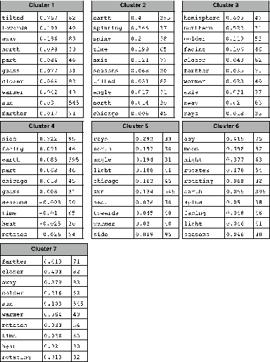
Figure 2. Words and their corresponding values in the centroid vectors.

I believe that the lists of words shown in Figure 2 are suggestive of clear meanings. For example, Cluster 1 seems to be about the tilt of the earth, while Cluster 7 is about something being closer or farther from a heat source (usually the sun).

Applying the cluster vectors to the transcripts

Once we have these “building blocks” we can use them to analyze each of the 54 transcripts. To do this, I first take each transcript, segment it as before, and compute vectors for each of these segments. Then I compare these vectors for segments to the vectors that correspond to each of the 7 cluster centroids.

When this is done for Edgar’s transcript, the results are as shown in Figure 3. In this analysis, the transcript has been broken into 10 segments. For each of these 10 segments, there are 7 bars, corresponding to the 7 cluster centroids. In the first part of the transcript, the bar corresponding to Cluster 5—the blue bar—dominates. This cluster has to do with rays striking the earth’s surface. Cluster 7 dominates in the latter half of the transcript. This is the cluster that has to do with being closer or farther from a source. Furthermore, this shift occurs at around the right time in the transcript.

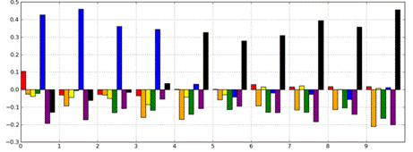
Figure 3. Segmenting analysis for Edgar.

The analysis for Zelda is a bit simpler. Cluster 1 dominates throughout the entire transcript. This is the cluster that has to do with the earth’s tilt. This makes sense since Zelda’s explanation was tilt-based. It is also important to note that the blue bar—Cluster 5—is comparatively high in some of the segments. This is the bar that has to do with rays striking the earth at an angle.

.

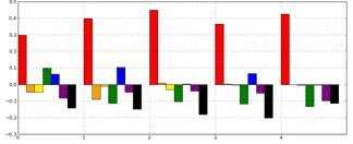
Figure 4. Segmenting analysis of Zelda's transcript.

Figure 5. Segmenting analysis of Caden's transcript.

The analysis for Caden makes an interesting contrast to the analysis for Zelda. We understood Caden as also giving a tilt-based analysis. As can be seen in Figure 5, Cluster 3 dominates in many of the segments. This has to do with the earth’s hemispheres. But Cluster 1 (tilt) and Cluster 7 (close and farther) also appear. This makes sense since Caden gave an explanation in which first one hemisphere, then the other, is tilted toward the earth. And unlike Zelda, Caden said that this tilting affects the earth’s temperature because one hemisphere will be closer to the sun (not because it received more directly sunlight). Thus, this analysis captures relatively subtle differences between these two tilt-based explanations.

Conclusion

I hope that the preceding analysis makes it clear that there are simple yet powerful computational methods that can capture the richness and diversity of student reasoning. They are conceptually simple—the algorithms involved can be described in just a few words, and they don’t rely on sophisticated mathematics. The algorithms are also easy to apply in a very practical sense, since there is publically available source code that can be drawn upon (as long as we are willing to work in Python). There is still some programming to be done. But all that is required is a few lines of programming to link together the publicly available code.

The analysis I presented here is a type of learning analytics. But hopefully it is clear that the methods I described can be used for more then determining if students are being efficiently channeled toward a desired end goal. They can be used to find commonalities across students (in the form of the building blocks), and they also allow us to capture more personal aspects of students explanatory constructions.

I worked with transcript data here. As I said earlier, I believe that the data employed in EDM and LA should ultimately incorporate more use of richer kinds of data, including spoken language and text.

I have only scratched the surface here of the types of methods that are available to us. I presented just one type of vector space model; there are many more sophisticated alternatives. And, within computational linguistics and machine learning, vector space models and clustering are just two examples drawn from a wide range of methods, many of which could be applied for similar purposes. (See, for example, Manning & Schütze, 1999.) I hope that in presenting just a single example analysis I have convinced the reader that it is possible to use computational methods to analyze data in a way that is consistent with the constructivist vision. It can be a force for good rather than evil.

References

Baker, R., Corbett, A., Roll, I., & Koedinger, K. (2008). Developing a generalizable detector of when students game the system. User Modeling and User-Adapted Interaction, 18(3), 287-314.

Bird, S., Klein, E., & Loper, E. (2009). Natural language processing with Python (1st ed.). Beijing ; Cambridge Mass.: O'Reilly.

Buckingham Shum, S., & Deakin Crick, R. (2012). Learning dispositions and transferable competencies: pedagogy, modelling and learning analytics. Paper presented at the 2nd International Conference on Learning Analytics & Knowledge,, Vancouver.

Long, P., & Siemens, G. (2011). Penetrating the Fog: Analytics in Learning and Education. EDUCAUSE review, 46(5), 30-41.

Manning, C. D., & Schütze, H. (1999). Foundations of statistical natural language processing. Cambridge, MA: MIT Press.

Papert, S. (1980). Mindstorms. New York: Basic Books.

Sherin, B. L., Krakowski, M., & Lee, V. R. (2012). Some assembly required: How scientific explanations are constructed during clinical interviews. Journal of Research in Science Teaching, 49(2), 166-198.